Mechanical regularization in EikoTwin DIC
- By Lucas Angénieux, Research engineer at EikoSim
In EikoTwin DIC, the measurement of displacement fields is performed on the simulation mesh. However, as this mathematical problem is by nature ill-posed, a mechanical regularization parameter allows the user to add mechanical conditions to the field measurements.
Contrary to most digital image correlation software, at EikoSim, we have chosen to use a mechanical “filter”. It allows not to filter the displacement field in an artificial way and to keep a mechanical meaning in the displacement field.
This article explains the meaning of this regularization and provides some recommendations for its use.
Why add mechanical regularization?
In digital image correlation (DIC), in order to compute the displacement fields from a set of images, we use the gray levels of a reference image and the following one to track the displacement between the two (more information in these articles about the basics of DIC and the global method).
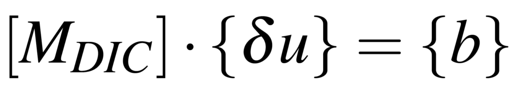
This hypothesis of gray levels conservation allows to build the minimization problem (1), put in matrix form:
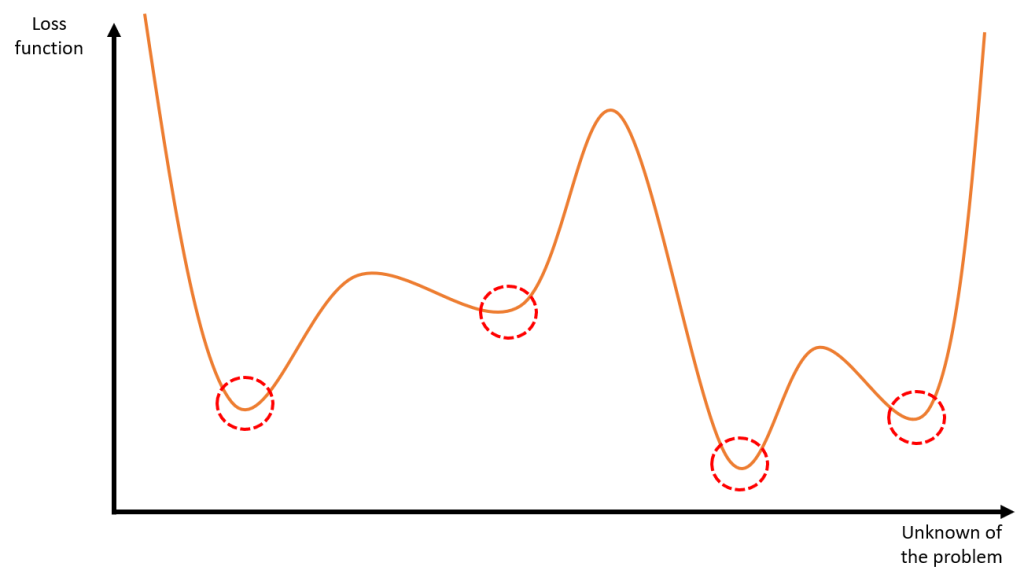
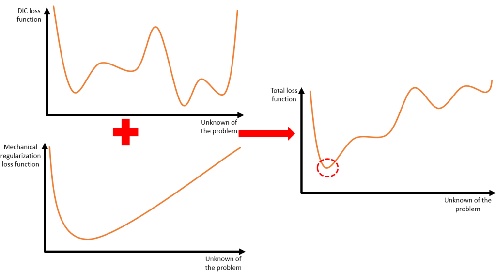
The Gauss-Newton type scheme used to solve this problem has good convergence characteristics but risks not converging to a satisfactory result if the loss function has many flat parts or local minima: the problem is ill-posed (see Figure 1).
We will therefore look for a way to modify this function to allow algorithm convergence despite these problematic areas.
One of the solutions used to solve complex problems is to use regularization. This technique consists of adding a penalization term to the loss function to be minimized to discard the solutions that least satisfy certain criteria expected on the resulting field.
In the case of mechanical regularization, it is the mechanically inadmissible displacement fields (for example, too “high frequency”) that will be penalized. This solution, which acts as a mechanical “filter”, can be close to filters used in most current DIC software, except that here, only mechanical assumptions are made.
Mechanical regularization in EikoTwin DIC
To add mechanical information to the problem, we can base ourselves on a solid constitutive equation with a simplified hypothesis that depends on the material considered.
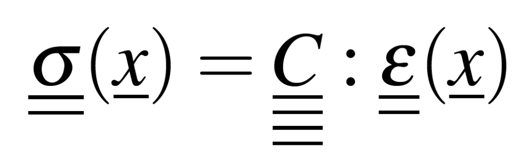
Except in the case of an architectural or multiphase material for example, we can choose Hooke’s law in linear, homogeneous, and isotropic elasticity (LHI), which will allow us to treat faithfully many industrial cases.
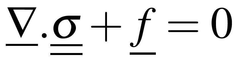
With Hooke’s law (2) and the static equilibrium of a solid (3), we then modify the scheme (1) into the following form (4):

Thus, the new system is equivalent to minimizing a new loss function, linear combination of the image correlation and regularization functions (see Figure 2). A weighting must be applied to these two functions in order to avoid a too important influence of one of these functions on the measured field. This is where the regularization length to be chosen by the user in EikoTwin DIC operates.
The regularization length in EikoTwin DIC
In EikoTwin DIC, the user chooses 3 parameters when launching the measurement of the displacement and strain fields: the maximum number of iterations, the convergence criterion, and the regularization length. The choice of this length has an influence on the results as well as on the convergence speed. It is then necessary to understand its physical meaning in order to make the best choice possible.
In the following, we will discuss different examples. These examples are based on virtually generated images using EikoTwin Virtual, a software developed by EikoSim (see the article on virtual testing with EikoTwin Virtual for more explanations). Thus, it is possible to generate relevant images for which we have full knowledge of the geometry and theoretical displacement and strain fields that will be used as references.
The regularization length is seen as the size of the local approximation area to a linear elastic model
As we have seen previously, mechanical regularization is based on a constitutive law: Hooke’s law in linear, homogeneous, and isotropic elasticity. Without mechanical regularization, the finite element formalism already imposes a continuity of the displacement from one node to another, during the measurement. Regularization allows us to add a mechanical hypothesis to a set of nodes locally.
Thus, the regularization length can be seen as the size of the local area in which the model is approximated by a linear elastic model. A regularization length that is too large will therefore limit the motion of the part to a rigid body motion, while a regularization length that is smaller than the size of an element will have absolutely no effect.
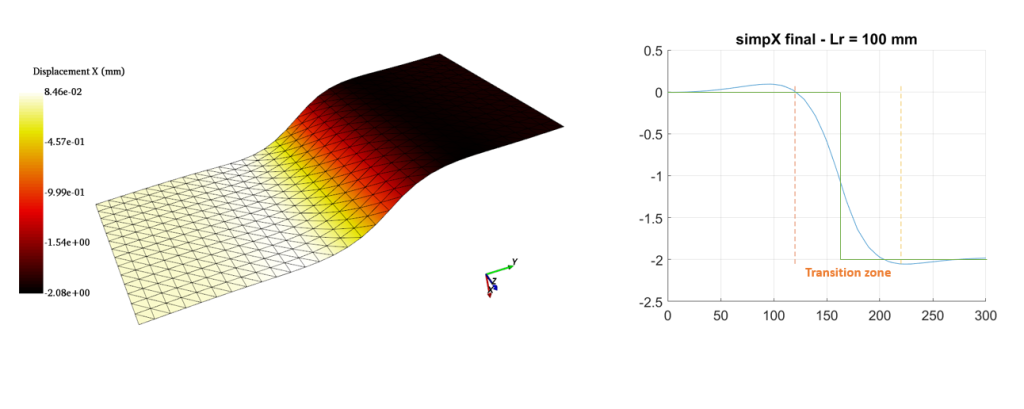
In the example of Figure 3, we observe a flat part with a displacement step of 2 mm along the normal to the part (in the graph on the right, the green curve represents the displacement profile applied to the part in the virtual images used in this example).
Here, the applied regularization length (100 mm) can be seen as the length over which the step from 0 to 2 mm will be measured. The graph on the right shows the displacement profile according to the normal, with a “transition zone” of 100 mm. This zone is the area where the effect of the linear elastic constitutive law seen previously is effectively visible.
In practice, one must be careful about not choosing a length of regularization too important compared to the orders of magnitude which one seeks to measure, not to lose the information contained in the initial measurement, potentially noisy (without the length of regularization).
The regularization length is seen as the cutoff frequency of a low-pass filter
One can also see the regularization length as a filter that cuts off high-frequency variations in the displacement field. In this context, the wavelength associated with the cutoff frequency is equal to the regularization length.
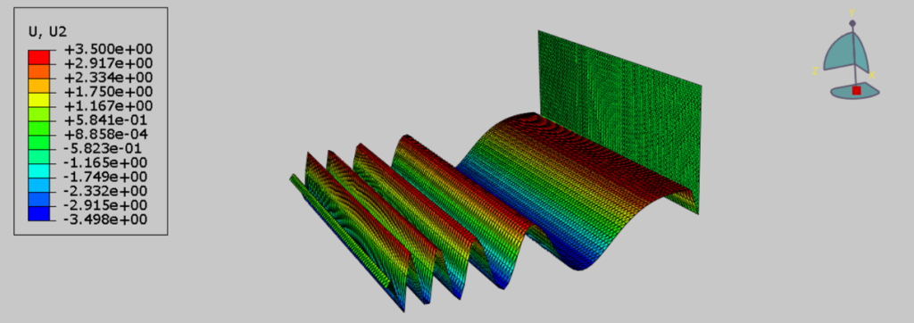
A relevant illustration of this vision is presented in Figure 4 below. Here we observe the case of an L-shaped mockup of 2000 mm. Virtual images of this mockup have been generated (using EikoTwin Virtual) following the profile of Figure 4: a pseudo-sinusoidal normal displacement along the Y-direction, of fixed amplitude whose wavelength varies continuously from 100 mm to 1500 mm along the length of the mockup. The elements have a size of about 60 mm.
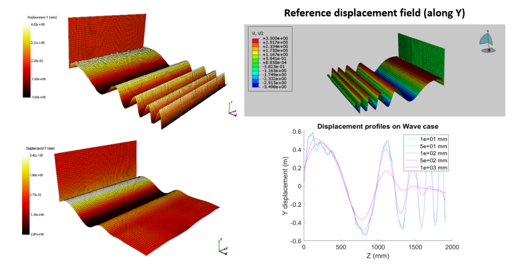
We then analyze the measured displacement field for different mechanical regularization lengths (from 50 mm at the top to 1000 mm at the bottom) in Figure 5. As expected, regularization has no effect for the lowest length (of a value smaller than the size of an element; the signal is noisy, but all displacement fluctuations have been measured).
For the highest regularization length (corresponding to half the size of the plate), there are no more very high-frequency fluctuations (“noise”) at the scale of the element (see in particular the zone close to the vertical plane); the wavelengths small in front of this 1000 mm length are clearly attenuated. Only the wave with a wavelength higher than 1000 mm is measured correctly.
On the right, the normal displacement profile along a line on the Z-axis of the part has been plotted. We can then observe the different displacement profiles according to the wavelength used, highlighting the regularization’s low-pass filter-like behavior.
Towards a more mathematical vision of mechanical regularization
Another way to see the influence and weight of the mechanical regularization in the problem (4) can be illustrated on Figure 6 below:
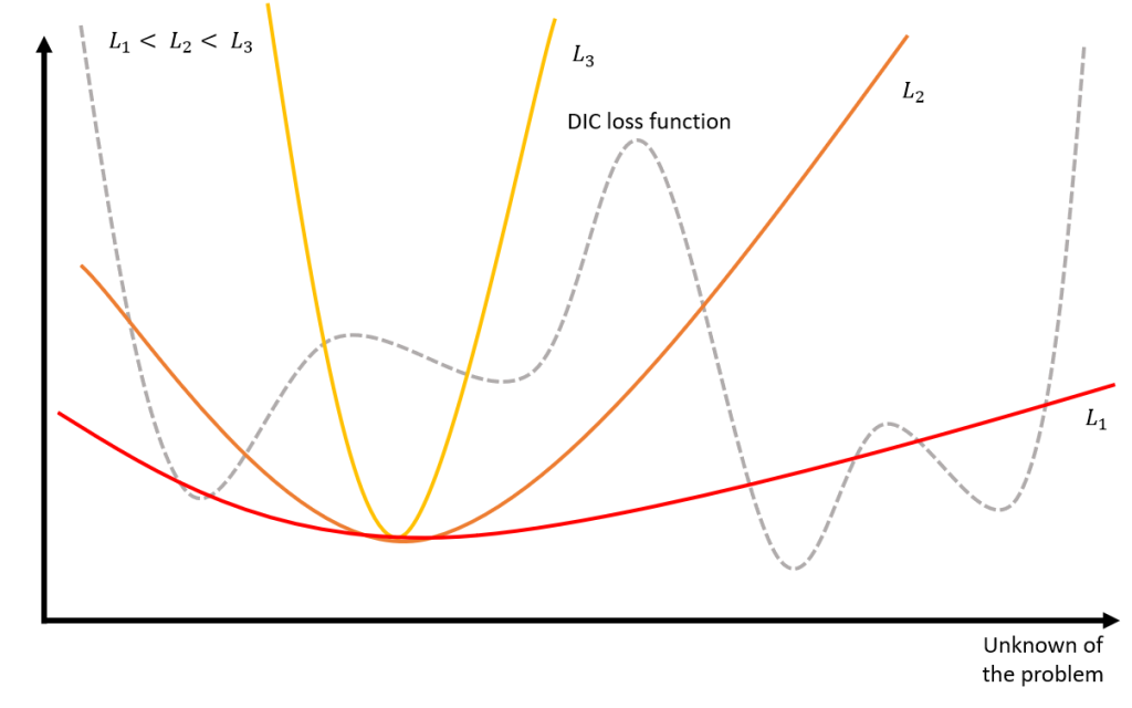
In Figure 6, we see that the regularization length has an influence on the mechanical regularization loss function [1]. Thus, in this example, the length L1 (too small) has very little influence on the total loss function, and there will remain local minima on the right that do not correspond to the solution. The algorithm might not converge correctly.
A too-high length L3 will give too much weight to the mechanical regularization and will therefore discriminate the global minimum solution. We see that the length L2 will displace the local minima on the right, and favor the minimum of the left which is the solution.
How to choose the right mechanical regularization length?
It is important to note that the regularization length depends on the case under study (mesh, measurement area, a phenomenon to be observed, etc…), and there is no “ideal” length in the absolute. It is up to the user to choose the most suitable regularization length for his particular case, by making the best compromise between computation speed, convergence and level of details (i.e. richness of the displacement field). This article allows in a first place to better understand the effect of mechanical regularization on the solution field and the physical meaning of the length to be applied.
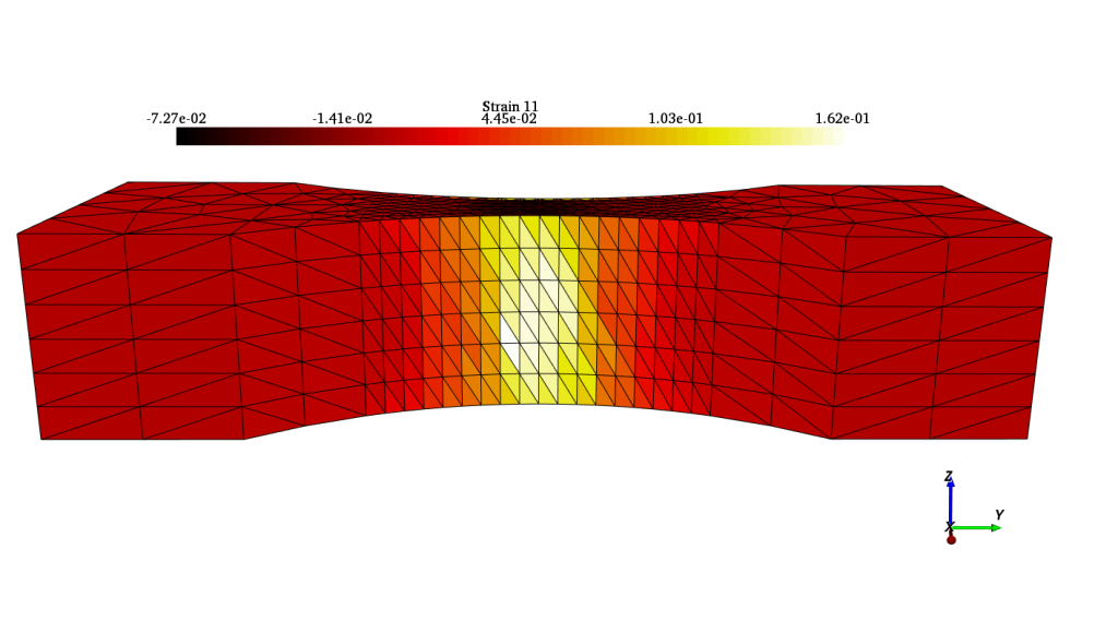
To illustrate this section, we will look at the strains measured on virtual images of a conventional tensile specimen, 95 mm long and meshed with 2 mm size elements in the area of interest. The reference strain field along the tensile axis (used for the generation of the images) is shown in Figure 7 below.
At EikoSim, we first recommend performing a full measurement without regularization. This provides preliminary results, without any mechanical regularization effect. In the second step, a regularization length of the size of 2 or 3 elements may be relevant to improve the convergence without measurement noise. An analysis of the effect of the regularization length on a particular quantity of interest (displacement sensor, strain gauge, etc…) or on the fields (displacements, strains, correlation residuals) can also help to refine this choice.
This is what we are going to do on the specimen in this example. In view of the solicitations and our images, it is more relevant to focus on the residuals and the strains in the middle of the specimen rather than on the displacement fields.
The residual fields are an efficient tool to judge the choice of the regularization length. The user can launch different measurements by increasing the length and study its influence on the residual field (the use of the Batch Mode plugin can be particularly relevant here). The regularization length will increase the residuals from a certain value, especially in the area where the part is the most deformed.
Indeed, the displacement field measured will be similar to a rigid body motion, and in this case, the contribution of the regularization term in the global function will be disproportionate. We can therefore study from what value we observe this local increase in residuals, especially in the areas of interest of our test.
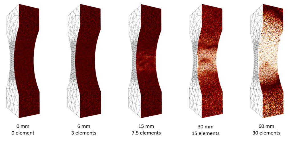
In our example, we can see in Figure 8 that from a regularization length of 15 mm, the residuals increase and even explode after 30 mm, a sign of a very bad measurement of the displacement field. It is, therefore advisable to choose a length between 0 and 10 mm (i.e., between 0 and 5 elements).
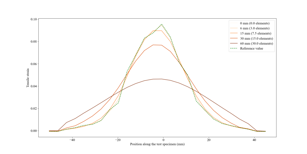
The tensile strain profile along the specimen can also be seen in Figure 9 (by plotting at a fixed time the strain along the tensile axis on a profile). In accordance with the explanation of the effect of regularization given above, the influence of the regularization length chosen by the user on the measurements made in EikoTwin DIC can be directly seen here. If the regularization length is too high, the fields will be smoothed and crushed, and the strain measured along the profile will decrease.
These profiles confirm the previous choice of 6 mm (i.e., 3 elements) regularization length compared to a 15 mm length. This case illustrates the interest in regularization (filtering of high frequencies interfering with the test results) while showing the negative impact that a choice of a too-high length can have. Particular attention must therefore be paid to the choice of the regularization length to make the best possible compromise between speed and convergence of the computation and the level of detail of the measurement.
Conclusion
In this article, we have seen that the mechanical regularization in EikoTwin DIC is a mathematical tool that imposes a mechanical condition on the measurement of fields by digital image correlation. Mechanical regularization allows correcting errors that can occur during some tests: simulation mesh too fine, speckle pattern not adapted to the size of the mesh, measurement noise too important, which prevents a correct interpretation of the results, etc…
The different physical or mathematical approaches of the regularization length help us understand its use better to obtain excellent results during tests. In practice, a first analysis without regularization, then a progressive evolution of this length by looking at the quantities of interest specific to the test, allows to choose the adapted regularization length. A length equal to the size of 2 or 3 elements is generally well-adapted in most cases.
Bibliographic references
[1] Arturo Mendoza, Jan Neggers, François Hild, Stéphane Roux. Complete Mechanical Regularization
Applied to Digital Image and Volume Correlation. Computer Methods in Applied Mechanics and
Engineering, Elsevier, 2019, 355, pp.27-43. 10.1016/j.cma.2019.06.005 . hal-02148780, Complete Mechanical Regularization Applied to Digital Image and Volume Correlation – Archive ouverte HAL (archives-ouvertes.fr)
98-100 AVENUE ARISTIDE BRIAND
92120 MONTROUGE
FRANCE