Measurement errors and digital image correlation
- By Pierre Baudoin, R&D engineer at EikoSim
When conducting a test campaign instrumented by digital image correlation, it must be possible to determine the characteristic measurement error for the quantities of interest studied (measured displacement or strain). This analysis is essential to know whether the measurement made is indeed the desired “signal” and not the measurement “noise”. All measurements must be related to this level of uncertainty, otherwise it is not possible to decide on their relevance. A specificity of digital image correlation is that the measurement error must be characterized at each new test. Indeed, it depends on many parameters that vary from one test to another (lighting, speckle, cameras and lenses used …). For clarification, this article proposes to present the errors that can be encountered on a digital image correlation test. It will also discuss how they can be quantified in order to validate a measurement result.
Random error et systematic error
The errors that can taint a measurement can be classified in two main categories (Fig. 1): random errors (measurement “noise”) and systematic errors (bias).
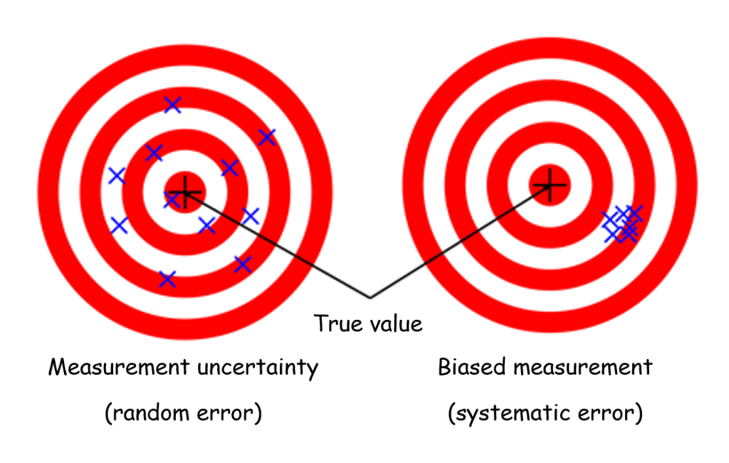
For a given quantity of interest, the random error (measurement uncertainty or « noise ») corresponds to the dispersion of the measured values around the measured mean. The main source of random error in digital image correlation is camera noise. This is the temporal fluctuation of the gray levels that each pixel of the camera sensor observing a fixed object will perceive.
The systematic error, also called bias, corresponds to a shift in the mean value of the measured signal from the mean value of the true signal. Sources of bias in digital image correlation measurements include incorrect calibration of the camera system or unintentional camera movement during the test. In the specific case of the global method, the choice of a regularization length that is too large in relation to the experimental strain gradient can also lead to a biased measurement. It should be noticed that while it is always possible to quantify random error (i.e. the dispersion of the experimental measurement), it is generally not possible to quantify the bias. Indeed, this bias is understood as a deviation from a true value that is unknown. Some exceptions are made for very special cases to which we will return in the last part of this article.
Calculation of uncertainty
The purpose of evaluating the « background noise » of the test is to determine the magnitude of the dispersion of the measured values for the quantity of interest under the test conditions. To characterize the signal dispersion, the simplest method is to take series of motionless images of the piece (without any imposed effort or displacement) under the test conditions and then process this series of images using the digital image correlation software. A « perfect » measurement would provide a zero-displacement field, at any points of the part and for all the processed images. However, since the noise disturbs the measurement, any deviation to zero in the measured fields is a measurement error.
It remains to characterize the amplitude of this noise, which is commonly done by calculating the standard deviation. In what follows, we will call Uij the displacement measured at node i for image j. For the sake of clarity, the component considered for the calculation will be omitted. However, the uncertainty calculations presented are to be performed and analyzed component by component. The approach will be identical for the estimation of the uncertainty on the components of the strain. We will start by calculating the nodal temporal standard deviation on all the nodes of the measurement mesh. This is given for node i by:
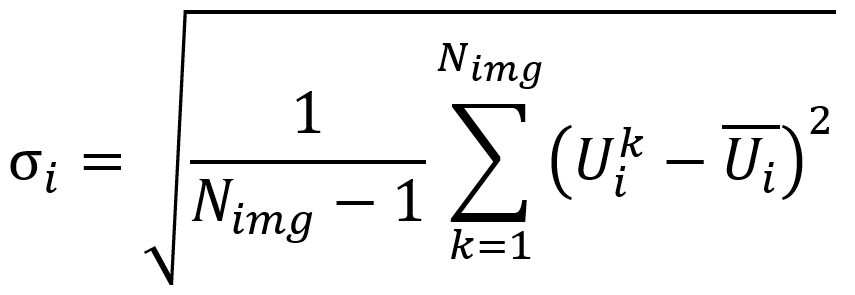
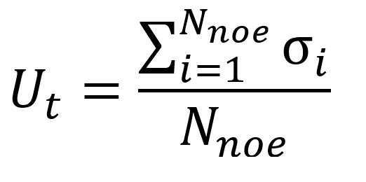
Where Nimg is the number of static images taken into account for the calculation of uncertainty, and ![]() the mean of the measured displacement at the node i over all the static images. The temporal uncertainty Ut is then deduced by taking the mean of these nodal temporal standard deviations over all the Nnoe nodes of the measurement mesh:
the mean of the measured displacement at the node i over all the static images. The temporal uncertainty Ut is then deduced by taking the mean of these nodal temporal standard deviations over all the Nnoe nodes of the measurement mesh:
An alternative metric encountered for these uncertainty calculations is that of spatial uncertainty. We first calculate the standard deviation of the displacement (or strain) for a single given image. That is to say the quantification of the dispersion of the displacement measured over all the nodes of the measurement mesh. Then we calculate the mean of this quantity over all the images processed.
These two estimates generally provide similar values. Therefore, they can be used to determine whether a quantity of interest would be measurable for a given experimental configuration. It is generally assumed that a correctly performed measurement correspond to the signal if its amplitude is greater than 3 times this uncertainty, otherwise the measurement is indistinguishable from the measurement noise.
Practical recommendations:
- Acquire at least ten static images under the exact same test conditions (cameras, lenses, lighting, temperatures, possible start-up of surrounding test machines, etc…);
- The image processing for the uncertainty calculation must be carried out under the exact same conditions as the test itself: same measurement field, same convergence criterion, same length of mechanical regularization if it used for the measurement;
- Point of attention: this method provides a lower bound of the measurement uncertainty. Indeed, the exact conditions of the test will always be different from those of static images. If possible, we should preferer measurement configurations where the quantity of interest is very large compared to the background noise (factor 3 or more). It might be necessary to adapt the experimental set-up (higher resolution of cameras, longer focal length). It is also possible to change the finite element model (coarser elements for instance) in order to reduce the uncertainty below the desired threshold for the intended application.
What about bias?
As a rule, it is not possible to determine this bias precisely. Indeed, the « true » value of the quantities of interest is unknown and is the subject of measurement. However, it is possible to exclude some sources of bias by performing some pre-testing.
In addition to the uncertainty study described in the previous section, another quantity may be of interest. Thus, we can analyse the evolution of the mean of the quantity of interest over a set of static images. A variation of this value over time or space will be sign of a bias due to camera movement, vibrations in the test hall… Sources that it will be up to the user to discriminate.
In the case of post-processing with EikoTwin DIC, some user parameters may introduce bias in the measurement. The first is the finite element mesh used to perform the measurement. If the elements are too large in relation to the characteristic size of the phenomenon to be observed, this introduces an artificial smoothing of the results which can lead to bias. This will generally not be the case when this mesh is the result of a well-designed finite element computation. Indeed, its aim is to described precisely the phenomenon that one wishes to validate with the test. However, this can happen when the mesh is created specifically for the measurement. In any case, the user must keep a critical eye on the adequacy of his mesh to the description of the observed phenomenon. Similarly, the case where a too fine mesh requires the use of a mechanical regularization can be problematic. Care must be taken to limit the length of regularization to a few elements. Indeed, this length is likely to introduce a bias in the measurement.
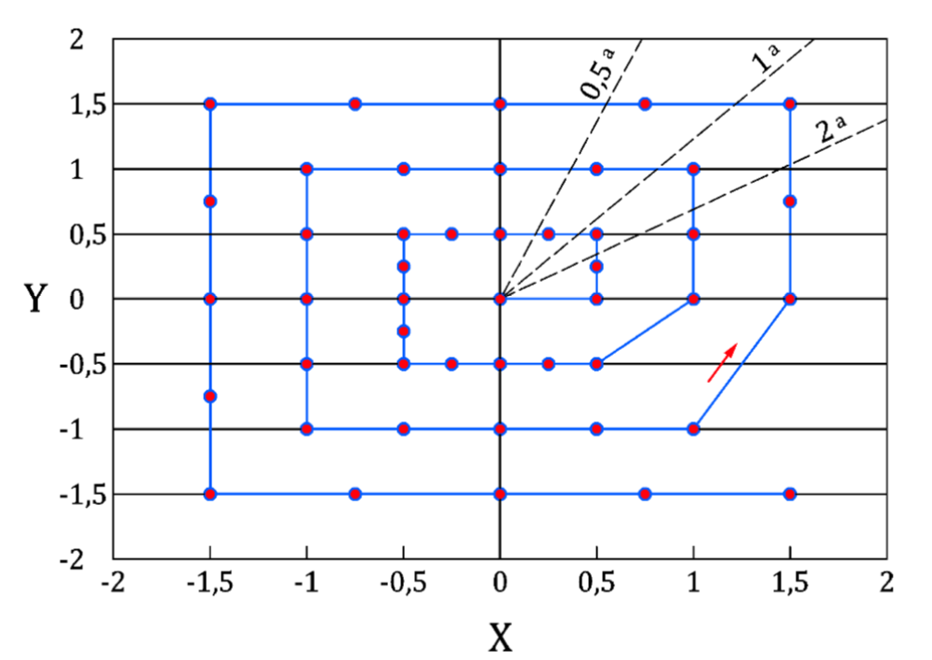
Finally, among the efforts made to characterize bias in digital image correlation, we can refer to the ASD-STAN prEN 4861 P1 standard which defines a procedure for measuring bias. The principle is to apply a series of known displacements (Figure 2) to the part under study and to determine the bias for each position of the object, which makes it possible to estimate the quality of the measurement for the entire study volume. However, this procedure cannot generally be applied to a testing device on structure. Indeed, it is necessary to be able to precisely move the part under study in its environment, which limits the adoption of this standard in practice.
Conclusion
Practical determination of the measurement error on a digital image correlation test presents several specific challenges. It should be remembered that the measurement error depends on many parameters specific to each test. We will return soon in a future blog article on the subject on these parameters. It is also desirable to acquire a series of static images before each test. Thus, it is possible to determine the amplitude of the measurement noise. It is the knowledge of these amplitudes that will determine the framework of a relevant test-simulation comparison. First of all, it must be ensured that the amplitude of the simulated quantity to be validated is much higher than the measurement noise. In a second step, a significant difference between test and simulation can only be demonstrated when the difference between measured and calculated quantities is higher than the measurement noise.
Finally, when writing the test reports, it is essential to document all the steps taken to quantify any uncertainties and biases, and to take these into account when interpreting the test results.
98-100 AVENUE ARISTIDE BRIAND
92120 MONTROUGE
FRANCE